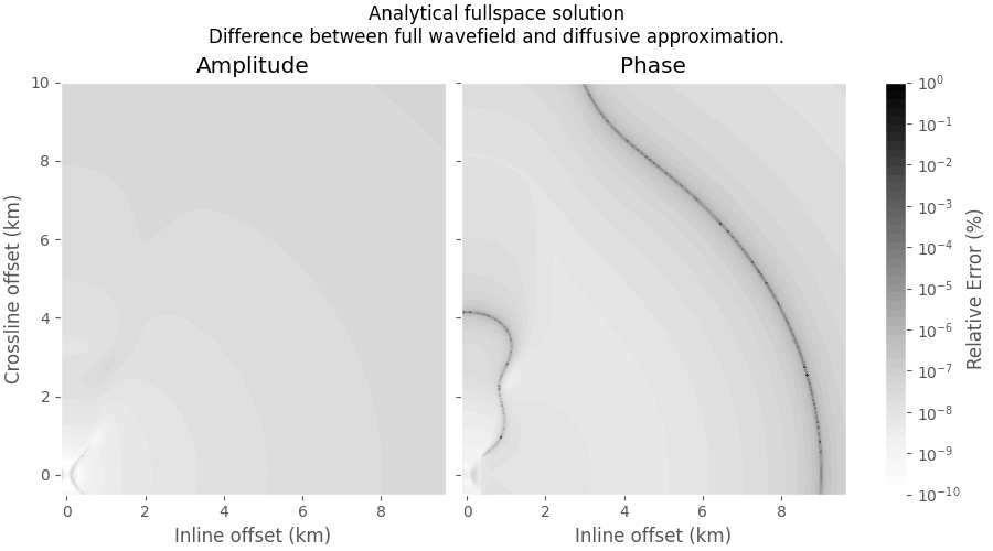
Full wavefield vs diffusive approximation for a fullspace

Example comparison of the electric field using the complete Maxwell’s equations, and the electric field using the diffusive or quasi-static approximation.

You can play around with the parameters to see that the difference is getting bigger for

• higher frequencies, and

• higher electric permittivity / magnetic permeability.

import empymod
import numpy as np
import matplotlib.pyplot as plt
plt.style.use('ggplot')

Define model

x = np.arange(526)*20. - 500
x[x == 0] += 1e-3  # Avoid warning message regarding 0 offset.
rx = np.tile(x[:, None], x.size)
ry = rx.transpose()
inp = {
    'src': [0, 0, 0],                     # Source [x, y, z]
    'rec': [rx.ravel(), ry.ravel(), 50],  # Receiver [x, y, z]
    'res': 1/3,                           # Resistivity
    'freqtime': 0.5,                      # Frequency
    'aniso': np.sqrt(10),                 # Anisotropy
    'ab': 11,                             # Configuration; 11=Exx
    'epermH': 1.0,                        # Electric permittivity
    'mpermH': 1.0,                        # Magnetic permeability
    'verb': 1,                            # Verbosity
}

Computation

# Halfspace
hs = empymod.analytical(solution='dfs', **inp).reshape(rx.shape)

# Fullspace
fs = empymod.analytical(**inp).reshape(rx.shape)

# Relative error (%)
amperr = np.abs((fs.amp() - hs.amp())/fs.amp())*100
phaerr = np.abs((fs.pha(unwrap=False) - hs.pha(unwrap=False)) /
                fs.pha(unwrap=False))*100

Plot

fig, (ax1, ax2) = plt.subplots(
        1, 2, figsize=(9, 5), sharey=True, constrained_layout=True)
fig.suptitle('Analytical fullspace solution\nDifference between full ' +
             'wavefield and diffusive approximation.')

# Min and max, properties
vmin = 1e-10
vmax = 1e0
props = {
    'levels': np.logspace(np.log10(vmin), np.log10(vmax), 50),
    'locator': plt.matplotlib.ticker.LogLocator(),
    'cmap': 'Greys',
}

# Plot amplitude error
ax1.set_title('Amplitude')
cf1 = ax1.contourf(rx/1000, ry/1000, amperr.clip(vmin, vmax), **props)
ax1.set_ylabel('Crossline offset (km)')

# Plot phase error
ax2.set_title('Phase')
cf2 = ax2.contourf(rx/1000, ry/1000, phaerr.clip(vmin, vmax), **props)

for ax in [ax1, ax2]:
    ax.set_xlabel('Inline offset (km)')
    ax.set_xlim(min(x)/1000, max(x)/1000)
    ax.set_ylim(min(x)/1000, max(x)/1000)
    ax.axis('equal')

# Plot colorbar
cb = plt.colorbar(cf2, ax=[ax1, ax2], ticks=10**np.arange(-10, 1.))
cb.set_label('Relative Error (%)')

empymod.Report()

Sat Jan 17 19:14:45 2026 UTC
OS	Linux (Ubuntu 22.04)	CPU(s)	2	Machine	x86_64
Architecture	64bit	RAM	7.6 GiB	Environment	Python
File system	ext4
Python 3.11.12 (main, May 6 2025, 10:45:53) [GCC 11.4.0]
numpy	2.3.5	scipy	1.17.0	numba	0.63.1
empymod	2.5.4.dev4+g4866dc83a	libdlf	0.3.0	IPython	9.9.0
matplotlib	3.10.8

Estimated memory usage: 359 MB