Note
Go to the end to download the full example code.
TEM: AEMR TEM-FAST 48 system#
In this example we compute the TEM response from the TEM-FAST 48 system.
This example was contributed by Lukas Aigner (@aignerlukas), who was interested in modelling the TEM-FAST system, which is used at the TU Wien. If you are interested and want to use this work please have a look at the corresponding paper Aigner et al. (2024).
The modeller empymod models the electromagnetic (EM) full wavefield Greens
function for electric and magnetic point sources and receivers. As such, it can
model any EM method from DC to GPR. However, how to actually implement a
particular EM method and survey layout can be tricky, as there are many more
things involved than just computing the EM Greens function.
What is not included in empymod at this moment (but hopefully in the
future), but is required to model TEM data, is to account for arbitrary
source waveform, and to apply a lowpass filter. So we generate these two
things here, and create our own wrapper to model TEM data. See also the example
TEM: ABEM WalkTEM, on which this example
builds upon.
References
Aigner, L., D. Werthmüller, and A. Flores Orozco, 2024, Sensitivity analysis of inverted model parameters from transient electromagnetic measurements affected by induced polarization effects; Journal of Applied Geophysics, Volume 223, Pages 105334, doi: 10.1016/j.jappgeo.2024.105334.
import empymod
import numpy as np
import matplotlib.pyplot as plt
from scipy.special import roots_legendre
from matplotlib.ticker import LogLocator, NullFormatter
from scipy.interpolate import InterpolatedUnivariateSpline as iuSpline
plt.style.use('ggplot')
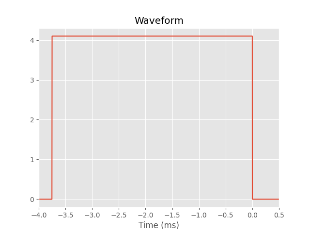
1. TEM-FAST 48 Waveform and other characteristics#
The TEM-FASt system uses a “time-key” value to determine the number of gates, the front ramp and the length of the current pulse. We are using values that correspond to a time-key of 5.
turn_on_ramp = -3.0E-06
turn_off_ramp = 0.95E-06
on_time = 3.75E-03

injected_current = 4.1  # Ampere
time_gates = np.r_[4.060e+00, 5.070e+00, 6.070e+00, 7.080e+00,
                   8.520e+00, 1.053e+01, 1.255e+01, 1.456e+01,
                   1.744e+01, 2.146e+01, 2.549e+01, 2.950e+01,
                   3.528e+01, 4.330e+01, 5.140e+01, 5.941e+01,  # time-key 1
                   7.160e+01, 8.760e+01, 1.036e+02, 1.196e+02,  # time-key 2
                   1.436e+02, 1.756e+02, 2.076e+02, 2.396e+02,  # time-key 3
                   2.850e+02, 3.500e+02, 4.140e+02, 4.780e+02,  # time-key 4
                   5.700e+02, 6.990e+02, 8.280e+02, 9.560e+02,  # time-key 5
                   ] * 1e-6  # from us to s

waveform_times = np.r_[turn_on_ramp - on_time, -on_time,
                       0.000E+00, turn_off_ramp]
waveform_current = np.r_[0.0, injected_current, injected_current, 0.0]

plt.figure()
plt.title('Waveform')
plt.plot(np.r_[-9, waveform_times*1e3, 2], np.r_[0, waveform_current, 0])
plt.xlabel('Time (ms)')
plt.xlim([-4, 0.5])
2. empymod implementation#
def waveform(times, resp, times_wanted, wave_time, wave_amp, nquad=3):
    """Apply a source waveform to the signal.

    Parameters
    ----------
    times : ndarray
        Times of computed input response; should start before and end after
        `times_wanted`.

    resp : ndarray
        EM-response corresponding to `times`.

    times_wanted : ndarray
        Wanted times.

    wave_time : ndarray
        Time steps of the wave.

    wave_amp : ndarray
        Amplitudes of the wave corresponding to `wave_time`, usually
        in the range of [0, 1].

    nquad : int
        Number of Gauss-Legendre points for the integration. Default is 3.

    Returns
    -------
    resp_wanted : ndarray
        EM field for `times_wanted`.

    """

    # Interpolate on log.
    PP = iuSpline(np.log10(times), resp)

    # Wave time steps.
    dt = np.diff(wave_time)
    dI = np.diff(wave_amp)
    dIdt = dI/dt

    # Gauss-Legendre Quadrature; 3 is generally good enough.
    # (Roots/weights could be cached.)
    g_x, g_w = roots_legendre(nquad)

    # Pre-allocate output.
    resp_wanted = np.zeros_like(times_wanted)

    # Loop over wave segments.
    for i, cdIdt in enumerate(dIdt):

        # We only have to consider segments with a change of current.
        if cdIdt == 0.0:
            continue

        # If wanted time is before a wave element, ignore it.
        ind_a = wave_time[i] < times_wanted
        if ind_a.sum() == 0:
            continue

        # If wanted time is within a wave element, we cut the element.
        ind_b = wave_time[i+1] > times_wanted[ind_a]

        # Start and end for this wave-segment for all times.
        ta = times_wanted[ind_a]-wave_time[i]
        tb = times_wanted[ind_a]-wave_time[i+1]
        tb[ind_b] = 0.0  # Cut elements

        # Gauss-Legendre for this wave segment. See
        # https://en.wikipedia.org/wiki/Gaussian_quadrature#Change_of_interval
        # for the change of interval, which makes this a bit more complex.
        logt = np.log10(np.outer((tb-ta)/2, g_x)+(ta+tb)[:, None]/2)
        fact = (tb-ta)/2*cdIdt
        resp_wanted[ind_a] += fact*np.sum(np.array(PP(logt)*g_w), axis=1)

    return resp_wanted
def get_time(time, r_time):
    """Additional time for ramp.

    Because of the arbitrary waveform, we need to compute some times before and
    after the actually wanted times for interpolation of the waveform.

    Some implementation details: The actual times here don't really matter. We
    create a vector of time.size+2, so it is similar to the input times and
    accounts that it will require a bit earlier and a bit later times. Really
    important are only the minimum and maximum times. The Fourier DLF, with
    `pts_per_dec=-1`, computes times from minimum to at least the maximum,
    where the actual spacing is defined by the filter spacing. It subsequently
    interpolates to the wanted times. Afterwards, we interpolate those again to
    compute the actual waveform response.

    Note: We could first call `waveform`, and get the actually required times
          from there. This would make this function obsolete. It would also
          avoid the double interpolation, first in `empymod.model.time` for the
          Fourier DLF with `pts_per_dec=-1`, and second in `waveform`. Doable.
          Probably not or marginally faster. And the code would become much
          less readable.

    Parameters
    ----------
    time : ndarray
        Desired times

    r_time : ndarray
        Waveform times

    Returns
    -------
    time_req : ndarray
        Required times
    """
    tmin = np.log10(max(time.min()-r_time.max(), 1e-10))
    tmax = np.log10(time.max()-r_time.min())
    return np.logspace(tmin, tmax, time.size+2)
def temfast(off_time, waveform_times, model, square_side=12.5):
    """Custom wrapper of empymod.model.bipole.

    Here, we compute TEM-FAST data using the ``empymod.model.bipole`` routine
    as an example. This function is based upon the Walk TEM example.

    We model the big source square loop by computing only half of one side of
    the electric square loop and approximating the finite length dipole with 3
    point dipole sources. The result is then multiplied by 8, to account for
    all eight half-sides of the square loop.

    The implementation here assumes a central loop configuration, where the
    receiver (1 m2 area) is at the origin, and the source is a
    square_side x square_side m electric loop, centered around the origin.

    Note: This approximation of only using half of one of the four sides
          obviously only works for central, horizontal square loops. If your
          loop is arbitrary rotated, then you have to model all four sides of
          the loop and sum it up.


    Parameters
    ----------
    off_time : ndarray
        times at which the secondary magnetic field will be measured

    waveform_times : ndarray
        Depths of the resistivity model (see ``empymod.model.bipole`` for more
        info.)

    depth : ndarray
        Depths of the resistivity model (see ``empymod.model.bipole`` for more
        info.)

    res : ndarray
        Resistivities of the resistivity model (see ``empymod.model.bipole``
        for more info.)

    square_side : float
        sige length of the square loop in meter.

    Returns
    -------
    TEM-FAST waveform : EMArray
        TEM-FAST response (dB/dt).

    """

    if 'm' in model:
        depth = model['depth']
        res = model
        del res['depth']
    else:
        res = model['res']
        depth = model['depth']

    # === GET REQUIRED TIMES ===
    time = get_time(off_time, waveform_times)

    # === GET REQUIRED FREQUENCIES ===
    time, freq, ft, ftarg = empymod.utils.check_time(
        time=time,          # Required times
        signal=1,           # Switch-on response
        ft='dlf',           # Use DLF
        ftarg={'dlf': 'key_601_2009'},
        verb=2,
    )

    # === COMPUTE FREQUENCY-DOMAIN RESPONSE ===
    # We only define a few parameters here. You could extend this for any
    # parameter possible to provide to empymod.model.bipole.
    hs = square_side / 2  # half side length
    EM = empymod.model.bipole(
        src=[hs, hs,   0, hs, 0, 0],  # El. bipole source; half of one side.
        rec=[0, 0, 0, 0, 90],         # Receiver at the origin, vertical.
        depth=depth,                  # Depth-model, including air-interface.
        res=res,                      # if with IP, res is a dictionary with
                                      # all params and the function
        freqtime=freq,                # Required frequencies.
        mrec=True,                    # It is an el. source, but a magn. rec.
        strength=8,                   # To account for 4 sides of square loop.
        srcpts=3,                     # Approx. the finite dip. with 3 points.
        htarg={'dlf': 'key_401_2009'},  # Short filter, so fast.
    )

    # Multiply the frequecny-domain result with
    # \mu for H->B, and i\omega for B->dB/dt.
    EM *= 2j*np.pi*freq*4e-7*np.pi

    # === Butterworth-type filter (implemented from simpegEM1D.Waveforms.py)===
    cutofffreq = 1e8                 # determined empirically for TEM-FAST
    h = (1+1j*freq/cutofffreq)**-1   # First order type
    h *= (1+1j*freq/3e5)**-1
    EM *= h

    # === CONVERT TO TIME DOMAIN ===
    delay_rst = 0                    # unknown for TEM-FAST, therefore 0
    EM, _ = empymod.model.tem(EM[:, None], np.array([1]),
                              freq, time+delay_rst, 1, ft, ftarg)
    EM = np.squeeze(EM)

    # === APPLY WAVEFORM ===
    return waveform(time, EM, off_time, waveform_times, waveform_current)
def pelton_res(inp, p_dict):
    """ Pelton et al. (1978).
    code from: https://empymod.emsig.xyz/en/stable/examples/time_domain/
               cole_cole_ip.html#sphx-glr-examples-time-domain-cole-cole-ip-py
    """

    # Compute complex resistivity from Pelton et al.
    # print('\n   shape: p_dict["freq"]\n', p_dict['freq'].shape)
    iwtc = np.outer(2j*np.pi*p_dict['freq'], inp['tau'])**inp['c']

    rhoH = inp['rho_0'] * (1 - inp['m']*(1 - 1/(1 + iwtc)))
    rhoV = rhoH*p_dict['aniso']**2

    # Add electric permittivity contribution
    etaH = 1/rhoH + 1j*p_dict['etaH'].imag
    etaV = 1/rhoV + 1j*p_dict['etaV'].imag

    return etaH, etaV
3. Computation non-IP#
depths = [8, 20]
rhos = [25, 5, 50]
model = {'depth': np.r_[0, depths],
         'res': np.r_[2e14, rhos]}

# Compute conductive model
response = temfast(off_time=time_gates, waveform_times=waveform_times,
                   model=model)
:: empymod END; runtime = 0:00:00.171964 :: 3 kernel call(s)
4. Computation with IP#
depths = [8, 20]
rhos = [25, 5, 50]
charg = np.r_[0, 0.9, 0]
taus = np.r_[1e-6, 5e-4, 1e-6]
cs = np.r_[0, 0.9, 0]

eta_func = pelton_res
depth = np.r_[0, depths]
model = {'depth': depth,
         'res': np.r_[2e14, rhos],
         'rho_0': np.r_[2e14, rhos],
         'm': np.r_[0, charg],
         'tau': np.r_[1e-7, taus],
         'c': np.r_[0.01, cs],
         'func_eta': eta_func}


# Compute conductive model
response_ip = temfast(off_time=time_gates, waveform_times=waveform_times,
                      model=model)
:: empymod END; runtime = 0:00:00.180262 :: 3 kernel call(s)
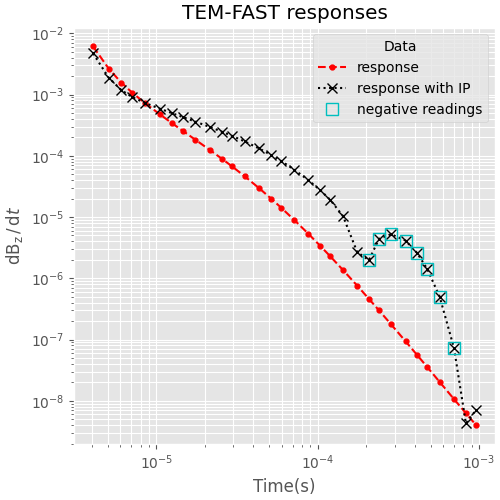
5. Comparison#
plt.figure(figsize=(5, 5), constrained_layout=True)

# Plot result of model 1
ax1 = plt.subplot(111)
plt.title('TEM-FAST responses')

# empymod
plt.plot(time_gates, response, 'r.--', ms=7, label="response")
plt.plot(time_gates, abs(response_ip), 'kx:', ms=7, label="response with IP")

sub0 = response_ip[response_ip < 0]
tg_sub0 = time_gates[response_ip < 0]
plt.plot(tg_sub0, abs(sub0), marker='s', ls='none',
         mfc='none', ms=8, mew=1,
         mec='c', label="negative readings")

# Plot settings
plt.xscale('log')
plt.yscale('log')
plt.xlabel("Time(s)")
plt.ylabel(r"$\mathrm{d}\mathrm{B}_\mathrm{z}\,/\,\mathrm{d}t$")
plt.grid(which='both', c='w')
plt.legend(title='Data', loc=1)


# Force minor ticks on logscale
ax1.yaxis.set_minor_locator(LogLocator(subs='all', numticks=20))
ax1.yaxis.set_minor_formatter(NullFormatter())
plt.grid(which='both', c='w')
empymod.Report()
Total running time of the script: (0 minutes 2.080 seconds)
Estimated memory usage: 227 MB