Note
Go to the end to download the full example code.
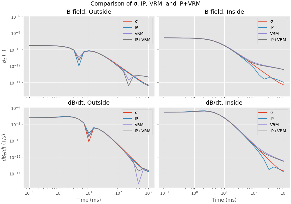
IP and VRM#
Induced Polarization (IP) and Viscous Remanent Magnetization (VRM): Comparison of responses of a model with only conductivities, IP, VRM, and IP+VRM.
This example is based on a contribution from Nick Williams (@orerocks).
import empymod
import numpy as np
import scipy as sp
import matplotlib.pyplot as plt
from scipy.constants import mu_0

plt.style.use('ggplot')
Survey Setup#
Loops#
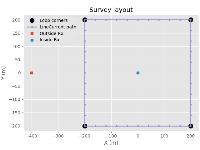
Create a square loop source of 400x400 m, and two Z-component receivers, one outside and one inside the loop; all at the surface (z=0).
# Create dipoles: [x0, x1, y0, y1, z0, z1]
src_x = np.r_[
    np.zeros(10), np.arange(10), np.ones(10)*10, np.arange(10, -1, -1)
]*40 - 200
src_y = np.r_[
    np.arange(10), np.ones(10)*10, np.arange(10, -1, -1), np.zeros(10)
]*40 - 200
src_bipole = [src_x[:-1],  src_x[1:], src_y[:-1], src_y[1:], 0, 0]

# Receiver locations: One outside, one inside; vertical
rec = [[-400., 0], [0, 0], [0, 0], 0, 90]

# Plot the loop
fig, ax = plt.subplots(constrained_layout=True)

# Source loop
ax.plot(src_x[::10], src_y[::10], 'ko', ms=10, label='Loop corners')
ax.plot(src_x, src_y, 'C2.-', lw=2, label='LineCurrent path')

# Receiver locations
ax.plot(rec[0][0], rec[1][0], 's', label='Outside Rx')
ax.plot(rec[0][1], rec[1][1], 's', label='Inside Rx')

ax.set_xlabel('X (m)')
ax.set_ylabel('Y (m)')
ax.set_title('Survey layout')
ax.legend()
ax.set_aspect('equal')
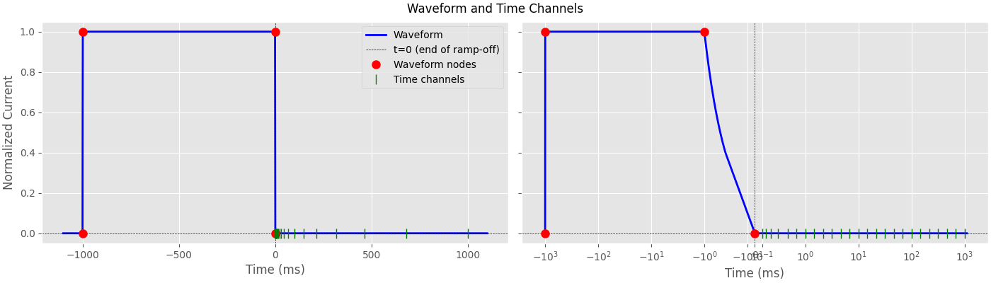
Trapezoid Waveform#
def current(times, nodes):
    """Small helper routine to get the waveform current for the given times."""
    # Off by default
    out = np.zeros(times.size)

    # Ramp on
    i = (times >= nodes[0]) * (times <= nodes[1])
    out[i] = (1.0 / (nodes[1] - nodes[0])) * (times[i] - nodes[0])

    # On
    i = (times > nodes[1]) * (times < nodes[2])
    out[i] = 1

    # Ramp off
    i = (times >= nodes[2]) * (times <= nodes[3])
    out[i] = 1 - (1.0 / (nodes[3] - nodes[2])) * (times[i] - nodes[2])

    return out


# On-time negative, t=0 at end of ramp-off
# Quarter period for 50 % duty cycle
source_frequency_hz = 0.25
on_time_s = 1 / (source_frequency_hz * 4)

# Time channels: off-time only, positive times
# 25 channels from 0.1 ms to 1000 ms for 0.25 Hz 50% duty cycle
times = np.logspace(-4, np.log10(on_time_s), 25)

# Waveform
nodes_times = np.array([-1, -0.999, -0.001, 0])
nodes_current = np.array([0., 1, 1, 0])
waveform_times = np.linspace(nodes_times[0] - 0.1, times[-1] + 0.1, 100000)
waveform_current = current(waveform_times, nodes_times)
print("Waveform details:")
print(
    f"  Time channels: {len(times)} channels from {times[0]*1000:.2f} ms to"
    f"{times[-1]*1000:.2f} ms (all off-time)"
)
print(
    f"  Waveform: on-time from {nodes_times[0]:.3f}s to"
    f"{nodes_times[3]:.3f}s"
)
print(f"    Ramp on: {nodes_times[0]*1e3:.3f} to {nodes_times[1]*1e3:.3f} ms")
print(f"    Ramp off: {nodes_times[2]*1e3:.3f} to {nodes_times[3]*1e3:.3f} ms")
print("  Off time: 0.000 ms")

# Plot waveform and time channels
fig, axs = plt.subplots(
        1, 2, figsize=(14, 4), sharey=True, constrained_layout=True)

for ax in axs:
    # Plot waveform
    ax.plot(waveform_times * 1e3, waveform_current, 'b-', linewidth=2,
            label='Waveform')
    ax.axhline(0, color='k', linestyle='--', linewidth=0.5)
    ax.axvline(0, color='k', linestyle='--', linewidth=0.5,
               label='t=0 (end of ramp-off)')

    # Mark waveform time nodes
    ax.plot(nodes_times * 1e3, nodes_current, 'ro', markersize=8,
            label='Waveform nodes', zorder=5)

    # Mark time channels
    ax.plot(times * 1000, np.zeros_like(times), 'g|', markersize=10,
            label='Time channels', zorder=10)

    # Formatting
    ax.set_xlabel('Time (ms)')

fig.suptitle('Waveform and Time Channels')
axs[0].set_ylabel('Normalized Current')
axs[0].legend()
axs[1].set_xscale('symlog', linthresh=0.4, linscale=0.5)
Waveform details:
  Time channels: 25 channels from 0.10 ms to1000.00 ms (all off-time)
  Waveform: on-time from -1.000s to0.000s
    Ramp on: -1000.000 to -999.000 ms
    Ramp off: -1.000 to 0.000 ms
  Off time: 0.000 ms
Waveform Functions#
These functions handle the trapezoid waveform convolution for the simulations. They are adapted from the WalkTEM example.
Key differences between B field and dB/dt:
For B field: bipole source strength is mu_0 * loop_current
For dB/dt: bipole source strength is loop_current, and we multiply by i*omega*mu_0 before frequency-to-time conversion
def get_time(time_channels, nodes_times):
    """
    Compute required times for waveform convolution.

    Because of the arbitrary waveform, we need to compute some times before and
    after the actually wanted times for interpolation of the waveform.

    time_req : ndarray
        Required times for computation (incl. extra points for interpolation)
    """
    t_log = np.log10(time_channels)
    # Add a point at the minimum time channel minus the time step, but don't go
    # lower than t=0 (end of ramp)
    tmin = np.max([t_log[0] - (t_log[1] - t_log[0]), -10])
    # Add a point at the maximum time channel plus the time step
    tmax = t_log[-1] + (t_log[-1] - t_log[-2])
    return np.logspace(tmin, tmax, time_channels.size + 2)
def apply_waveform_to_signal(
        times, resp, time_channels, wave_times, wave_amp, nquad=3):
    """
    Apply a source waveform to the signal.

    Modified from empymod WalkTEM example.
    """
    # Interpolate on log.
    PP = sp.interpolate.InterpolatedUnivariateSpline(np.log10(times), resp)

    # Wave time steps.
    dt = np.diff(wave_times)
    dI = np.diff(wave_amp)
    dIdt = dI / dt

    # Gauss-Legendre Quadrature; 3 is generally good enough.
    g_x, g_w = sp.special.roots_legendre(nquad)

    # Pre-allocate output.
    resp_wanted = np.zeros_like(time_channels)

    # Loop over wave segments.
    for i, cdIdt in enumerate(dIdt):
        # We only have to consider segments with a change of current.
        if cdIdt == 0.0:
            continue

        # If wanted time is before a wave element, ignore it.
        ind_a = wave_times[i] < time_channels
        if ind_a.sum() == 0:
            continue

        # If wanted time is within a wave element, we cut the element.
        ind_b = wave_times[i + 1] > time_channels[ind_a]

        # Start and end for this wave-segment for all times.
        ta = time_channels[ind_a] - wave_times[i]
        tb = time_channels[ind_a] - wave_times[i + 1]
        tb[ind_b] = 0.0  # Cut elements

        # Gauss-Legendre for this wave segment.
        logt = np.log10(np.outer((tb - ta) / 2, g_x) + (ta + tb)[:, None] / 2)
        fact = (tb - ta) / 2 * cdIdt
        resp_wanted[ind_a] += fact * np.sum(np.array(PP(logt) * g_w), axis=1)

    return resp_wanted
def convert_freq_to_time(EM, freq, time, ft, ftarg, time_channels, nodes_times,
                         waveform_current, compute_B_field=True):
    """
    Convert frequency-domain response to time domain and apply waveform.

    Parameters
    ----------
    EM : ndarray
        Frequency-domain EM response
    freq : ndarray
        Frequencies
    time : ndarray
        Time array for conversion
    ft : str
        Transform type
    ftarg : dict
        Transform arguments
    time_channels : ndarray
        Desired output times
    nodes_times : ndarray
        Waveform time nodes
    waveform_current : ndarray
        Waveform current values at time nodes
    compute_B_field : bool
        If True, compute B field (T). If False, compute dB/dt (T/s).

    Returns
    -------
    resp_wanted : ndarray
        Time-domain response at time_channels
    """
    if not compute_B_field:
        # For dB/dt: multiply by i*omega*mu_0 to convert H to dB/dt in
        # frequency domain
        EM *= 2j * np.pi * freq * mu_0

    # Convert to time domain
    delay_rst = 0
    EM, _ = empymod.model.tem(EM[:, None], np.array([1]), freq, time +
                              delay_rst, 1, ft, ftarg)
    EM = np.squeeze(EM)

    # Apply waveform
    return apply_waveform_to_signal(time, EM, time_channels, nodes_times,
                                    waveform_current)
Viscous Remanent Magnetization (VRM) Function#
This function implements VRM modeling, which is supported but not computed
within empymod.
def vrm_from_mu(inp, p_dict):
    """
    Isotropic VRM hook for empymod using mu-per-layer.
    Implements a log-uniform relaxation distribution over [tau1, tau2].

    Inputs expected in `inp` (all per-layer arrays):
    - mu    : baseline permeability (absolute). Exp. to be pre-mult. by mu_0
    - dchi  : amplitude of viscous susceptibility (dimensionless)
    - tau1  : lower bound of relaxation times [s]
    - tau2  : upper bound of relaxation times [s]
    """
    # Frequencies (nf,)
    freq = np.atleast_1d(p_dict["freq"])
    jw = 2j * np.pi * freq[:, None]

    # Per-layer inputs (nl,)
    mu = np.atleast_1d(inp["mu"])  # required
    dchi = np.atleast_1d(inp.get("dchi", 0.0))
    tau1 = np.atleast_1d(inp.get("tau1", 1e-10))
    tau2 = np.atleast_1d(inp.get("tau2", 10.0))

    # Log-uniform increment term
    ln_ratio = np.log(tau2[None, :] / tau1[None, :])
    incr = (1.0 - np.log((1.0 + jw * tau2[None, :]) /
            (1.0 + jw * tau1[None, :])) / ln_ratio)

    # Frequency-dependent relative permeability and zeta
    zeta = jw * (mu[None, :] + mu_0 * dchi[None, :] * incr)

    return zeta, zeta  # Horizontal and vertical the same
Cole-Cole Function#
This function implements Cole-Cole IP modeling, which is supported but not
computed within empymod. For more info on the Pelton model refer to the
IP example.
def pelton_cole_cole_model(inp, p_dict):
    """
    Pelton et al. (1978) Cole-Cole IP model.

    Inputs expected in `inp`:
    - res   : DC resistivity (Ohm-m)
    - m     : intrinsic chargeability (V/V), 0 <= m < 1
    - tau   : time constant (s)
    - c     : frequency dependency, 0 < c < 1

    Returns complex electrical conductivity (etaH, etaV).
    """
    # Compute complex resistivity from Pelton et al.
    iotc = np.outer(2j * np.pi * p_dict["freq"], inp["tau"]) ** inp["c"]
    # Version using equation 16 of Tarasov & Titov (2013)
    rhoH = inp["res"] * (1 + (inp["m"] / (1 - inp["m"])) * (1 / (1 + iotc)))
    rhoV = rhoH * p_dict["aniso"] ** 2

    # Add electric permittivity contribution
    etaH = 1 / rhoH + 1j * p_dict["etaH"].imag
    etaV = 1 / rhoV + 1j * p_dict["etaV"].imag

    return etaH, etaV
Custom empymod routine for IP and VRM#
def simulate_empymod(inp, res, times, compute_B_field=True, loop_current=1.0,
                     apply_vrm=False, apply_cole_cole=False):
    """
    Simulate TDEM response using empymod with trapezoid waveform. Supports VRM
    and Cole-Cole IP modeling.
    """
    # Get required times for computation
    time = get_time(times, nodes_times)

    # Get required frequencies
    time, freq, ft, ftarg = empymod.utils.check_time(
        time=time,
        signal=-1,  # Switch-off response
        ft="dlf",
        ftarg={"dlf": "key_81_2009"},
        verb=inp.get('verb', 0),
    )

    # Source strength depends on output field type
    # For B field: mu_0 * current returns B in frequency domain
    # For dB/dt: just current, then multiply by i*omega*mu_0 later
    strength = mu_0 * loop_current if compute_B_field else loop_current

    # Build empymod model dict with VRM and/or Cole-Cole hooks as needed
    res_dict = {"res": res}

    if apply_vrm:
        res_dict = {**res_dict, "func_zeta": vrm_from_mu, **apply_vrm}

    if apply_cole_cole:
        res_dict = {**res_dict, "func_eta": pelton_cole_cole_model,
                    **apply_cole_cole}

    # Compute frequency-domain response (summed over source elements)
    EM_loop = empymod.model.bipole(
        **inp,
        res=res_dict,
        freqtime=freq,
        signal=None,
        mrec=True,
        strength=strength,
        epermH=np.r_[0.0, np.ones(len(res)-1)],
        msrc=False,
        srcpts=3,
        htarg={"dlf": "key_101_2009", "pts_per_dec": -1},
    ).sum(axis=-1)

    # Convert to time domain and apply waveform
    nrec = EM_loop.shape[1]
    responses = np.zeros((nrec, times.size))

    for i_rx in range(nrec):
        responses[i_rx, :] = convert_freq_to_time(
            EM_loop[:, i_rx], freq, time, ft, ftarg, times, nodes_times,
            nodes_current, compute_B_field=compute_B_field
        )

    return responses
Subsurface Model#
inp = {
    'res': np.array([2e14, 1.0, 100]),
    'times': times,
    'inp': {
        'src': src_bipole,
        'rec': rec,
        'depth': [0.0, -50.0],
        'verb': 1,
    }
}

apply_cole_cole = {
    'm': np.array([0.0, 0.05, 0.15]),
    'tau': np.array([0.0, 0.005, 0.02]),
    'c': np.array([0.0, 0.4, 0.6]),
}

apply_vrm = {
    'dchi': np.array([0.0, 0.005, 0.02]),
    'mu': np.array([mu_0, mu_0 * 1.05, mu_0]),
}
Compute responses#
# Store results and timing for each model
results = {}

for compute_B_field in [True, False]:

    inp['compute_B_field'] = compute_B_field

    out = {}

    # Conductivity
    out['σ'] = simulate_empymod(**inp)
    # IP
    out['IP'] = simulate_empymod(**inp, apply_cole_cole=apply_cole_cole,)
    # VRM
    out['VRM'] = simulate_empymod(**inp, apply_vrm=apply_vrm)
    # IP + VRM
    out['IP+VRM'] = simulate_empymod(
            **inp, apply_cole_cole=apply_cole_cole, apply_vrm=apply_vrm)

    results["B field" if compute_B_field else "dB/dt"] = out
Plot results#
fig, axs = plt.subplots(
    2, 2, figsize=(10, 7), sharex=True, sharey=True, layout='constrained'
)

in_out = ['Outside', 'Inside']

# Loop over B-field - dB/dt
for i, compute_B_field in enumerate(["B field", "dB/dt"]):
    result = results[compute_B_field]

    # Loop over outside - inside loop
    for ii in range(2):

        # Loop over cases
        for k, v in results[compute_B_field].items():
            axs[i, ii].loglog(times*1e3, np.abs(v[ii, :]), label=k)

        axs[i, ii].set_title(f"{compute_B_field}, {in_out[ii]}")
        axs[i, ii].legend()

for ax in axs[1, :]:
    ax.set_xlabel('Time (ms)')
axs[0, 0].set_ylabel("$B_z$ (T)")
axs[1, 0].set_ylabel("$dB_z/dt$ (T/s)")

plt.suptitle("Comparison of σ, IP, VRM, and IP+VRM", fontsize=14)
plt.show()
empymod.Report()
Total running time of the script: (0 minutes 3.382 seconds)
Estimated memory usage: 211 MB